Excel Gantt Chart Template Conditional Formatting
Excel Formula Gantt Chart Exceljet
Excel Conditional Formatting Gantt Chart My Online

Excel Gantt Chart By Conditional Formatting Ver 2 Beat

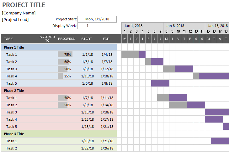
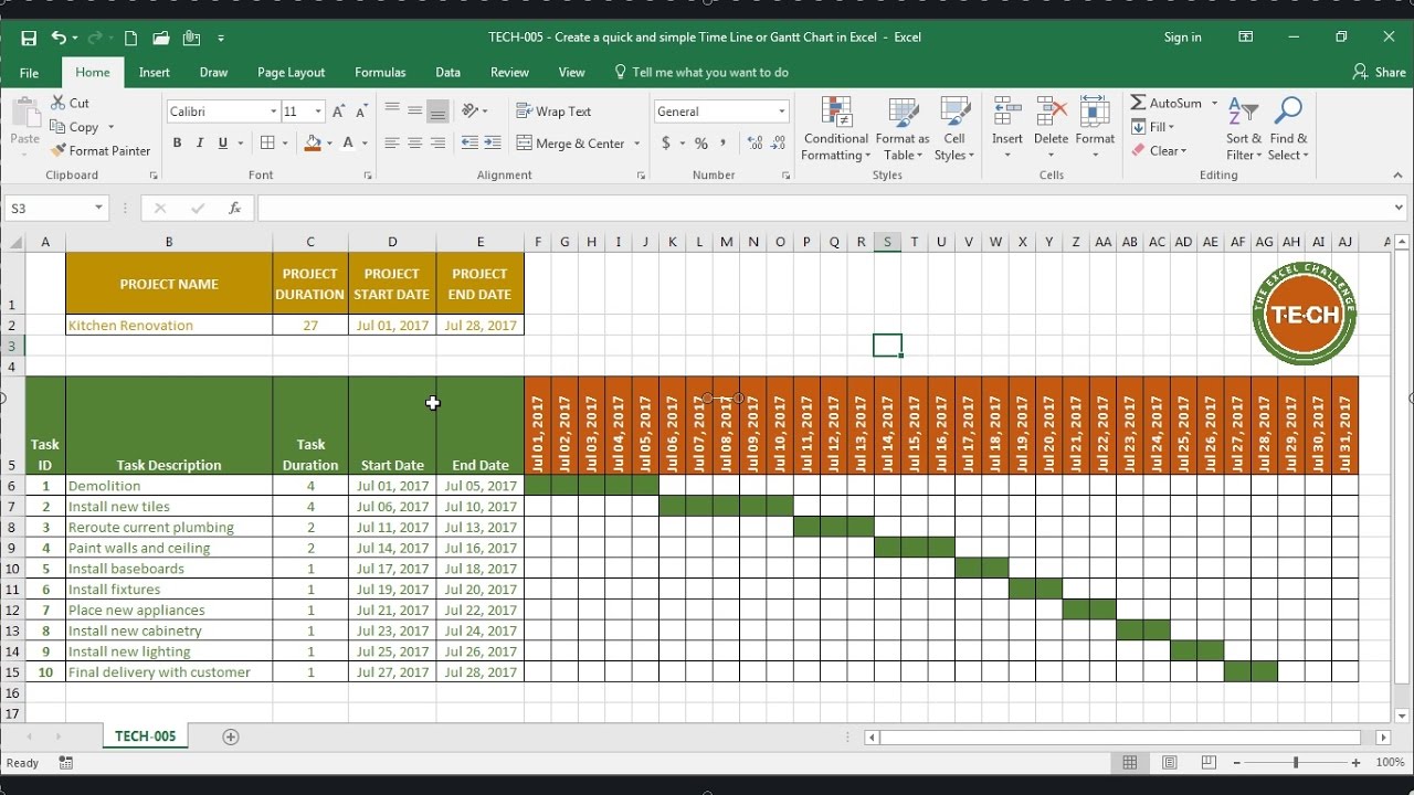
Excel Gantt Chart Template For Tracking Project Tasks

How To Build A Gantt Chart In Excel Critical To Success
Excel Conditional Formatting Gantt Chart My Online
2 for the horizontal axis.
Excel gantt chart template conditional formatting. Weekday d4 2 5 note. Start by selecting the range of cells where bars are to be displayed. A true outcome applies the format whereas false doesnt. There has to be 3 columns for jobs start date and job duration.
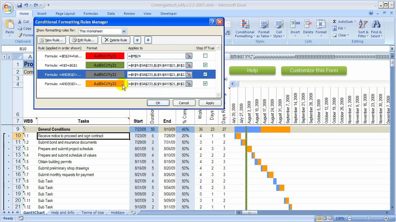
Our excel gantt chart with conditional formatting has taken advantage of some of the best tools in excel to create a powerful project management tool that will help you keep your next project on time and on budget. Here are the steps. Now click the format button and. Then in the new formatting rule dialog select use a formula to determine which cells.
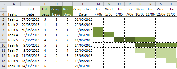
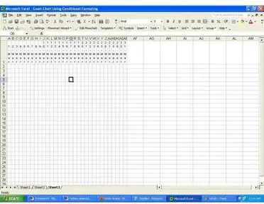
Select the cells which are in the date columns d2z7 and click home conditional formatting. 1 we need to make a layout for our chart. Pick new rule then choose a formula to determine which cells to format. We are going to use conditional formatting to make a gantt chart in this tutorial.
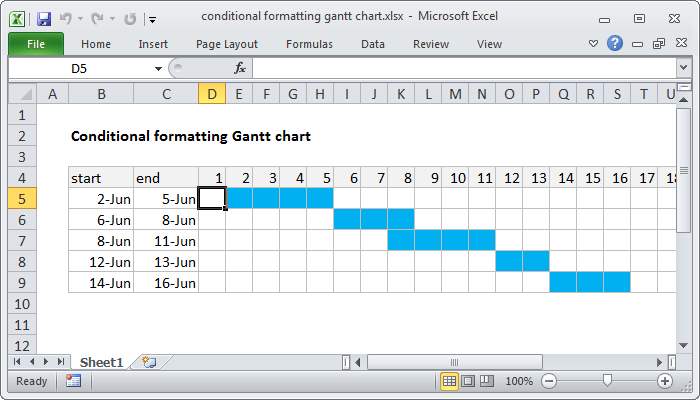
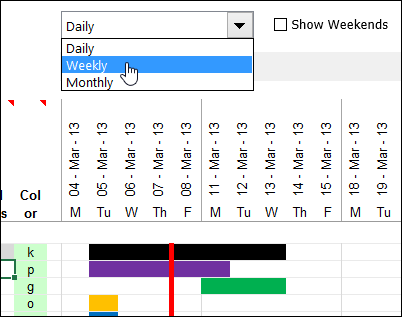
Supposing your data list as below screenshot shown. To build a gantt chart with weekends shaded you can use conditional formatting with a formula based on the weekday functionin the example shown the formula applied the calendar starting at d4 is. In the above example range f2t11. The conditional format will be copied to the entire range of the gantt chart and you will end up with a chart that looks like this one.
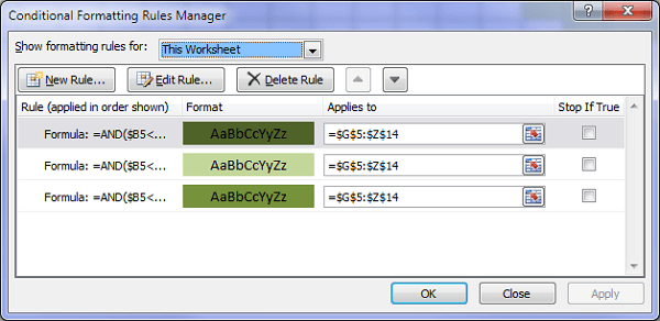
As you can see there are only 3 rules which are applied to the date columns gz. Conditional formatting applied data range conditional formatting is a great tool and lets you easily create gantt type charts right on the worksheet. Conditional formatting for gantt charts. This will make our vertical axis.
Click ok ok the gantt chart has been.
Simple Gantt Chart By Vertex42
Change Colors In Gantt Chart In Excel Workbook

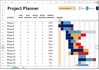
How To Build An Automatic Gantt Chart In Excel

Excel Gantt Chart Template

How To Use Conditional Formatting To Create A Gantt Chart In
Tech 005 Create A Quick And Simple Time Line Gantt Chart In Excel
Excel Gantt Chart Template Giveaway Contextures Blog
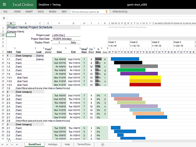
New Gantt Chart For Excel Online

Pin By Rich Mantz On Cadbimcomputer Gantt Chart Data
Excel Enthusiasts November 2016

Excel Formula Gantt Chart By Week Exceljet
Excel Gantt Chart Free Excel Templates

Project Manager Gantt Chart Professionalexcel Com

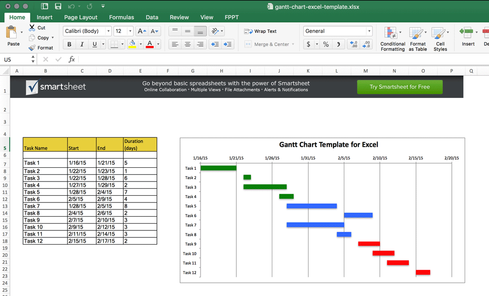
Free Gantt Chart Templates In Excel Other Tools Smartsheet
5 Gantt Chart Templates Excel Powerpoint Pdf Google
